Sampling

Source:

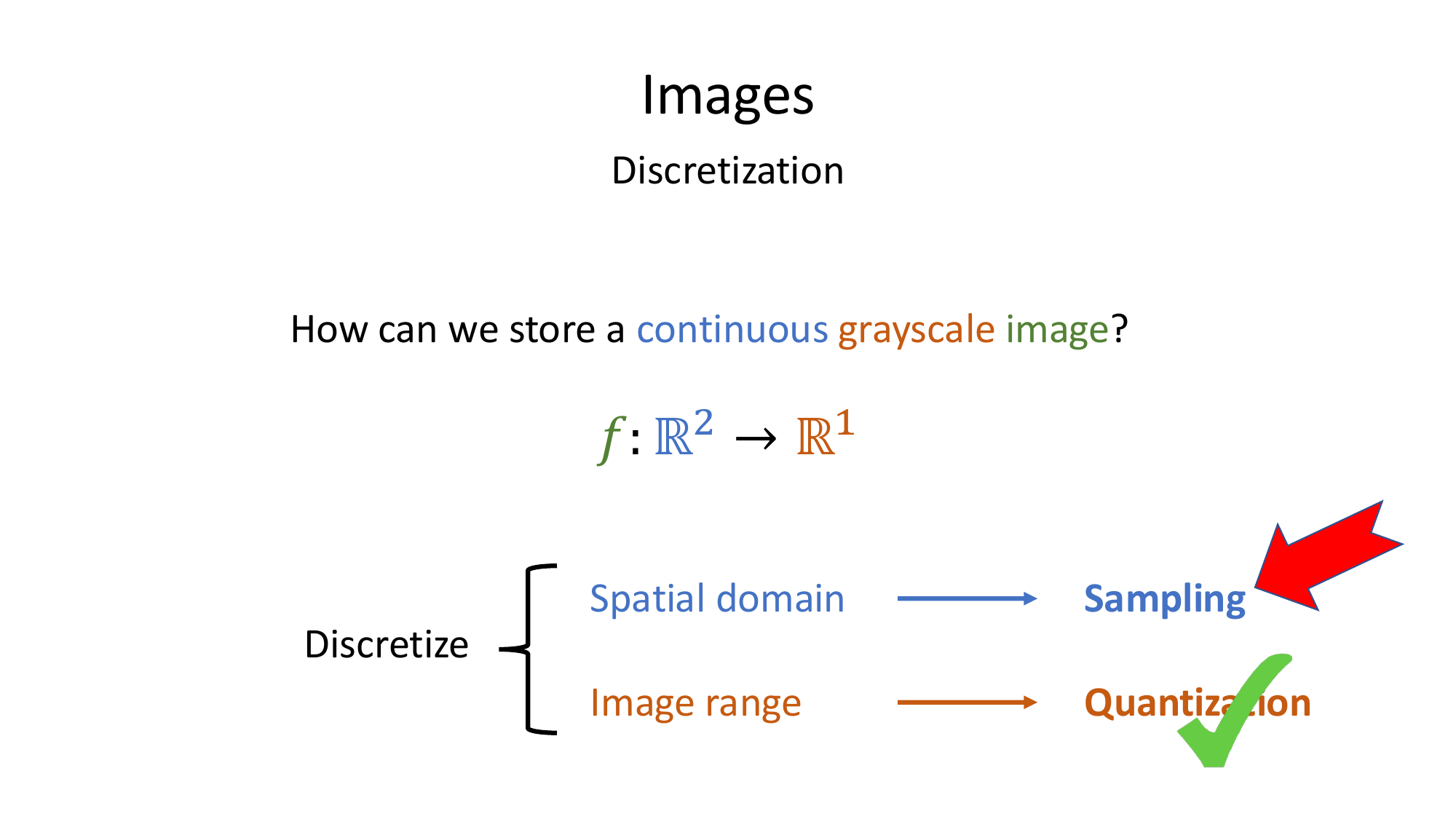
What sampling means

Sampling means:

choose specific positions where we measure the image

The original image is modeled as continuous:

f : R^{2} \to R_{+}

After sampling, we get a discrete image:

F : Z^{2} \to R_{+}

The lecture writes this as:

F (i, j) = f (i Δ y, j Δ x)

where:

Usually, we take:

Δ x = Δ y = 1

after choosing pixel coordinates.

Sampling is like placing graph paper over a smooth image and only reading the value at the grid points.

If the grid is:

If the samples are too far apart, small image details can disappear or be misrepresented.

That is why the slides mention the image should be “well sampled”.

Real cameras do not measure a perfect mathematical point.

A sensor element measures light over:

So a pixel value is closer to an average measurement than an exact point value.

The Remarkable notes add an important tradeoff:

So sampling is not only about spacing between grid points, but also about the effective area of each sensing probe.

The handwritten notes also record the common image-index convention:

If you sample every other location in 1D:

f (x) \to F (k) = f (2 k)

then you threw away half the positions immediately.